SPAM DETECTION – Natural Language Processing – in web

Ever wondered how are your emails and messages classified as spam or inbox? Of course, if you’ve come to go through this article you know it, right! It is done by training the machine on the basis of the collected data set. This is what is Natural Language Processing (NLP), programming computers to understand, interpret, and manipulate human language.

After studying this article you’ll definitely be able to create your own program to classify your messages.

Classifier Algorithm: Naive Bayes Algorithm

Interface:  Google Colabs 

Language Used: Python

So, without wasting much of our time let us head directly into spam detection. 

Spam is any kind of unwanted, unsolicited digital communication, that gets sent out in bulk. It is a huge waste of time and resources. Opposite of spam is ‘Ham’, which is a more technical term and will be used throughout the content.

Let’s have a look at the flow chart for the same.

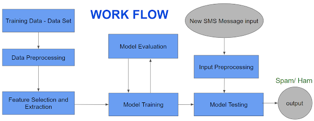
Step 1: First of all we need to have data set for training the model, you could easily get one from Kaggle or can download one directly from the given link (https://drive.google.com/file/d/1p_JAsEnpDjvBtVdcecrJnOIwAn3ne776/view?usp=sharing)

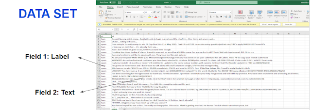
Here’s a sneak peek into the data set.

 

Step 2: Now comes data preprocessing, or data cleaning. It is an extremely important step to maintain the accuracy of the model, as the data set may contain some unwanted characters or blank rows etc.

Step 3: Basically we extract the data and divide it into the training and testing parts. Now training part is always more than the testing part, so we’ve kept 80% of the portion as training while 20% as the testing data set.

Step 4: After model training, model evaluation takes place and the model is being tested. Also, if we want we could input user data here and process it to get the result.

Let us first have a look at the code and then we’ll understand the working of the algorithm used. The following code can be directly executed on google collabs.

#Import libraries

import numpy as np 

import pandas as pd 

import nltk

from nltk.corpus import stopwords

import string

Why importing these? What are they used for? Wait… before more questions come, here’s the quick answer:

numpy: It is a python library used to perform mathematical operations on multidimensional objects as in array or matrices.

pandas: It is an open-source package which is used to read data from various kind of sources, CSV file(comma separated file) in our case.

nltk: Natural Language Tool Kit, It is a set of libraries for Natural Language Processing that helps in computer-human interaction.

stopwords: stopwords are the words used in an English sentence that do not add any specific meaning to it, so removing these words from our message won’t decrease the accuracy of our model. 

#Load the data

from google.colab import files # Use to load data on Google Colab

uploaded = files.upload() # Use to load data on Google Colab

You need to upload your dataset after this.

!ls

data = pd.read_csv('spam.csv', encoding='ISO-8859-1')

data.head(10)

#Print the shape (Get the number of rows and cols)

data.shape

#Get the column names

data.columns

 

you could view the details of your dataset using the above commands. Let’s now head towards data preprocessing.

 

#Checking for duplicates and removing them

data.drop_duplicates(inplace = True)

 

#Show the new shape (number of rows & columns)

data.shape

 

#Show the number of missing data for each column

data.isnull().sum()

 

#Need to download stopwords

nltk.download('stopwords')

def process_text(text):

    

#1 Remove Punctuationa

nopunc = [char for char in text if char not in string.punctuation] nopunc = ''.join(nopunc)

    

#2 Remove Stop Words

clean_words = [word for word in nopunc.split() if word.lower() not in stopwords.words('english')]

    

#3 Return a list of clean words

return clean_words

 

After preprocessing we move towards feature selection and extraction:

 

#Show the Tokenization (a list of tokens )

data['v2'].head().apply(process_text)

 

#convert the text into matrix of tokens

from sklearn.feature_extraction.text import CountVectorizer

messages_bow = CountVectorizer(analyzer=process_text).fit_transform(data['v2'])

 

#Split data into 80% training & 20% testing data sets

from sklearn.model_selection import train_test_split

X_train, X_test, y_train, y_test = train_test_split(messages_bow, data['v1'], test_size = 0.20, random_state = 0)

 

#Get the shape of messages_bow

messages_bow.shape

 

Now, after classification, we’ve started with data training.

 

# importing and training multinomial naive bayes for discrete values

from sklearn.naive_bayes import MultinomialNB

classifier = MultinomialNB().fit(X_train, y_train)

 

#Print the predictions

print(classifier.predict(X_train))

 

#Print the actual values

print(y_train.values)

 

#Evaluate the model on the training data set

from sklearn.metrics import classification_report,confusion_matrix, accuracy_score

pred = classifier.predict(X_train)

print(classification_report(y_train ,pred ))

print('Confusion Matrix: \n',confusion_matrix(y_train,pred))

print()

print('Accuracy: ', accuracy_score(y_train,pred))

 

#Print the predictions

print(classifier.predict(X_test))

#Print the actual values

print(y_test.values)

 

#Evaluate the model on the test data set

from sklearn.metrics import classification_report,confusion_matrix, accuracy_score

pred = classifier.predict(X_test)

print(classification_report(y_test ,pred ))

print('Confusion Matrix: \n',confusion_matrix(y_test,pred))

print()

print('Accuracy: ', accuracy_score(y_test,pred))

 

Each and every step of the code is explained in the comment along with it, you could also have a look at the Collaboratory here. (https://colab.research.google.com/drive/1GT7rZKXx4dMQj3CuarTAy2ZVnXSTXDwT?usp=sharing)

 

Coming to the algorithm now, we have used the Multinomial Naïve Bayes algorithm. It is used when the data is multinomial distributed, primarily used for document classification problems.

Given below is a quick look at the working of the algorithm:

 

Step 1: Convert the given dataset into frequency tables. The classifier uses the frequency of words for the predictors; hence a frequency table is being created for the given set of words.

 

Step 2: The likelihood table is generated by finding the probabilities of given features. It is nothing but the sum of probabilities divided by the total no of events.

Step 3: Now Bayes’ theorem is used to calculate the posterior probability. The posterior probability is the probability of occurrence of A when B has already occurred, where B is taken from the likelihood table.

 

Wondering about why we used Bayes’ theorem?

One of the main reason for using this algorithm is that all have studied Bayes’ theorem in our syllabus and it’s way easy to understand this, while the technical reasons sand out here:

• Naïve Bayes is one of the fast and easy ML algorithms to predict a class of datasets.

• It can be used for Binary as well as Multi-class Classifications.

• It performs well in Multi-class predictions as compared to the other Algorithms.

• It is the most popular choice for text classification problems.

• The accuracy of our model using the theorem stands out to be 99.2% on average.

Note: One of the major limitations of the model is that all features are independent or unrelated, so it cannot learn the relationship between features.

Hope you guys grabbed something from here. For a more detailed explanation of the theorem do visit Javatpoint. (https://www.javatpoint.com/machine-learning-naive-bayes-classifier)

Sanchita Mishra(2019-2023)

Computer Science Department

KIET Group of Institutions